
This is a revised version of this post: Warning: Excel can get Volatile
Excel is a great tool for dashboard/report delivery and design (it’s why we created our addin in the first place!), but there is a hidden performance trap:
Offset, Now, Today, Cell, Indirect, Info and Rand
If you’ve ever used any of these formulae, you may have noticed that whenever you change a cell, or collapse/expand a data grouping, Excel recalculates. That is because these are VOLATILE formulae, as soon as you use one of these, Excel will enter a mode where everything is always recalculating, and for good reason.
Offset & Now are the formulae we see used most often. Let’s look at each of these in turn and talk about some alternate approaches to avoid this issue.
Offset
This is by far the most common of these danger formulae that we see in use. Here’s the formula definition:
=Offset(reference,rows,cols,height,width)
Returns a reference to a range that is a specified number of rows and columns from a cell or range of cells. The reference that is returned can be a single cell or a range of cells. You can specify the number of rows and the number of columns to be returned.
Microsoft, OFFSET Function
Example – Dynamic Ranges
We typically see these as part of a named range definition for driving chart source data – it allows the number of rows/columns driving the chart data to change automatically; a not unusual requirement when it comes to building reports (especially when a report contains some user defined filters or slicers). Here’s an example:
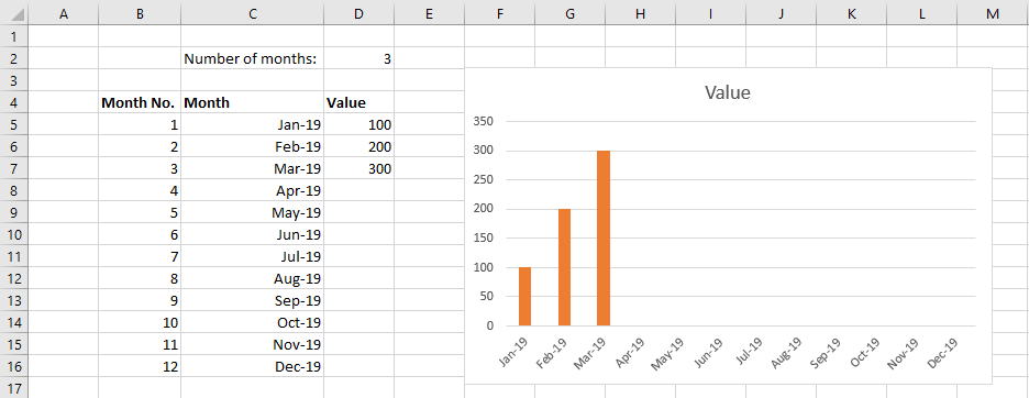
A very simple spreadsheet – we can type the number of months to display in the chart. In reality the number of months to display will probably be driven by the data available for the criteria selected. The screenshot already shows the issue we have – the chart is setup to display a max of 12 months, but we only have 3 months of data available.
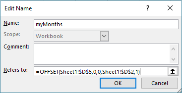
The most obvious approach is to use the Offset formula to pick the chart area to use automatically, we could create a named range such as:
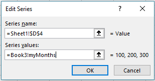
Now we just change the chart data source to be the named range:
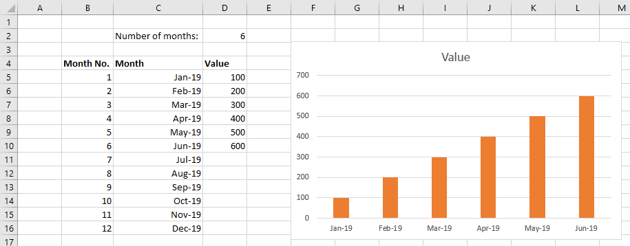
The chart is now plotting 3 months, but will automatically update to show the required number of months:
BUT we have now used a volatile formula – although this is a simple workbook, we are now in a position where Excel is going to have to recalculate everything all the time. It’s probably a good time to look at why Excel is going to do that. Let’s have a look at very simple formula to understand how Excel recalculates things.
What’s Happening?
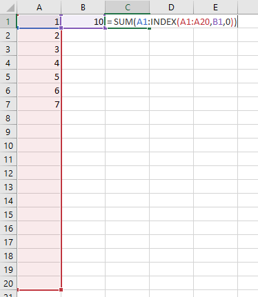
Consider the formula:
C1 = A1 + B1
We can see that C1 is dependent upon A1 & B1 – so whenever a value in either of these cells changes C1 will need to be recalculated to show the correct answer. Excel knows about this dependency because it maintains a dependency tree; it knows which cells need to be recalculated whenever any other cell changes. This is a very efficient way of working, if a workbook has thousands of formula, but only one values changes, and this only needs 10 of these formula to recalculate, then only 10 will be calculated.
If C1 contained:
C1 = SUM(A1:A20)
We know that C1 depends upon any of the cells A1:A20, and so does Excel. But what if C1 was:
C1 = SUM(OFFSET(A1,0,0,B1,1))
Which cells is C1 dependent upon? At a glance you could say A1 & B1.
But B1 contains the number 10, so actually C1 is dependent upon A1:A20 and B1 (the additional cells that are dependent are highlighted):

Just as we can’t see at a glance which cells C1 needs – Excel also can’t easily decide that. Therefore, Offset is volatile – if it wasn’t then there is a danger that Excel would take so long to work out if it needs to be calculated that it might as well always calculate it.
The Solution
There is an easy solution to this, INDEX. Here’s the formula definition (be careful, there are 2 ways to use Index, we want the REFERENCE one):
=INDEX(reference, row_num, [column_num], [area_num])
Returns the reference of the cell at the intersection of a particular row and column. If the reference is made up of non-adjacent selections, you can pick the selection to look in.
Microsoft, INDEX function
The big difference, compared to Offset, is that Index is going to return a single cell reference, so you need to use it as part of a range selection A1:Index(…). Here’s the same “Offset” Sum redefined as an “Index”:
C1 = SUM(A1:INDEX(A1:A20,B1,0))
The formula is simply saying the range we want starts at A1 and goes down the number of rows set in B1. The crucial difference is that the Index functions knows that A1:A20 is the maximum range we are likely to look at and therefore the dependencies are known just by looking at the formula itself:
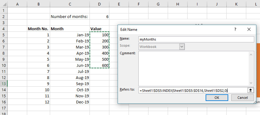
We can now update the Named Range to use the Index function instead:
=Sheet1!$D$5:INDEX(Sheet1!$D$5:$D$16,Sheet1!$D$2,0)
Now/Today
The Now and Today functions return the current date to a cell – this is generally used so that when a report is loaded it will always show the data based on “Today”. Whilst this is not an unreasonable thing to want to do, in reality what most people want is for the report to run for the most recent data, which could actually mean a number of things:
- Yesterday (if the data is built in a nightly process)
- The last working day (if the source transactional system is only used during office hours)
- Current month etc.
The easiest solution is to let the data determine the date to use – we can retreive this through an XLCubed grid, slicer or formula.
Grids – Reverse Sorting Members
If we use an XLCubed Grid or Query Table to retrieve the data, we can simply setup a grid to retrieve all days/months where there is data, then sort it in reverse order (so the most recent is at the top).
And use the Sort option “Reverse” to display the most recent data first:
With the grid set to “Refresh on Open” we know that A6 will always have the most recent date available in the cube and can base the rest of the report off that cell.
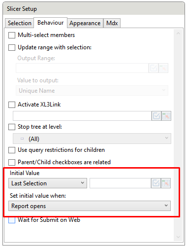
Slicers – Open On Last Selection
Slicers can be configured so that their initial value is the last available selection, i.e. the latest available date in a date hierarchy.
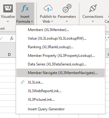
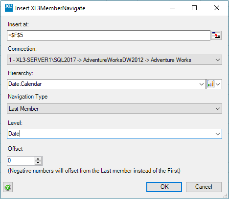
XL3MemberNavigate
The Xl3MemberNavigate formula can be used to retrieve the last member of a hierarchy at a particular level. There is a helpful wizard which can be access from the XLCubed ribbon.
This formula also allows you to include an offset. This means you could use one formula to retrieve the last available member (e.g. today’s date) and a second formula which retrieves the last available member with an offset of one (e.g. yesterday’s date).
Other Options
In some cases, retrieving the last member from a hierarchy does not work in getting today’s date, such as when the hierarchy contains future dates. In this situation, it is usually best to create the set of current/previous days in the cube. You can then pick this set in a slicer etc. If you can’t create the set in the cube you could use an Custom Calculation to do the same thing.


